In this post, I will be transforming raw Stock Market trading data into refined machine-learning-ready data that can be used to predict the price change for the next trading day. For example, will AAPL go up 1% or down 3% tomorrow?
Using data science principles, we will engineer technical indicators that will be used as features to train the machine learning model. For example, open-close percent change and simple moving averages. Additionally, we will transform the dataset from single-point observations into a time series. We will wrap it up by evaluating our model so that it can provide a benchmark for future revisions and enhancements.
As you may have guessed already, I will be using Scikit-Learn, Python, Pandas, and Numpy. If you don’t already have them then I suggest downloading the full package from Anaconda which conveniently installs everything in one go. Set up instructions can be found here – Data Science Like a Pro: Anaconda and Jupyter Notebook on Visual Studio Code.
See my Github repository for the full project including data and Jupyter Notebook.
The Data
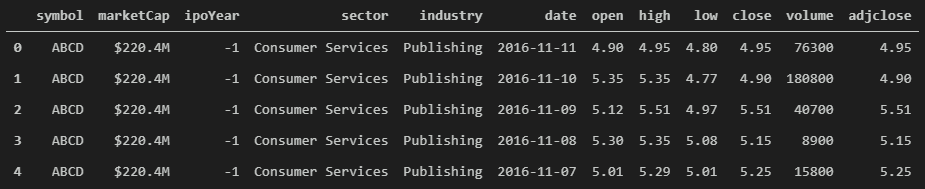
I pulled the daily data from the Yahoo API (before it was taken down) and combined it with Nasdaq data to bring in features like Market Cap, IPO Year, etc. One of my future posts will cover where and how to pull your own stock data including how to store it locally in a database. For now, my Github contains sample data.
Some questions about the data:
- Which column is the target vector? We will need to create it!
- How will features in the sample help predict the target vector? We will need to chain together several days of trading into one observation so that the model can learn based on patterns.
Clean Up
For the sake of simplicity, I will assume this will only be done with one company and only keep features that change day to day such as: date, open, high, low, close, volume, and adjclose.
# keep only relevant columns
data = data[['date', 'open', 'high', 'low', 'close', 'volume', 'adjclose']]
Technical Indicators
I’ll start by adding the first technical indicator and target vector: open-close percent change. To create this series we can use Pandas vector operations such as:
# add feature for percent change between open and close
data['percentChange'] = data['close'] / data['open'] - 1
data.head()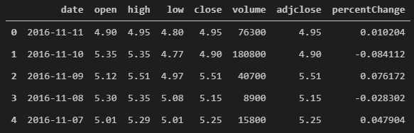
Once we have our target vector we can start to engineer new features that help us model the relationship between features and target vector. For example, for observation #1 – 2016-11-11, how does open, high, low, close, volume, adjclose correlate with the percent change? It’s a direct function of the features. In the real world, if we want to predict the next day we will not have its opening and closing price!
Let’s continue by creating a new feature based on the previous trading day’s percent change.
# create new feature for the percent change of the previous trading day
data['percentchange-1'] = data['percentChange'].shift(-1)
data.head()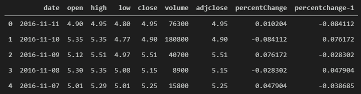
Now let’s try that again to get the percent change from two days ago.
# let's repeat again to get the previous percent change
data['percentchange-2'] = data['percentChange'].shift(-2)
data.head()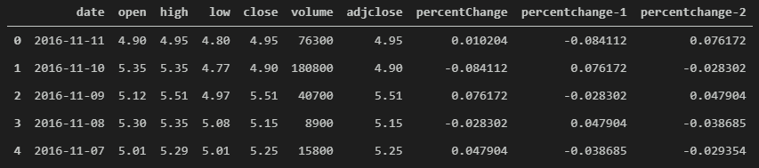
Notice how the data is evolving from what happened during the isolated trading day to what happened in the days leading to that day. We can repeat this process to bring in ‘n’ number of previous percent changes so that the machine learning algorithm can learn how trends correlate with the target vector.
Before calculating the simple moving average, we first need to sort the data with the oldest date on top. Try skipping this step before calculating SMA and you will notice that there is no way to change forward-looking vs backward-looking SMA calculations.
# reorder to have oldest date at top
# this is useful for creating rolling calculations
data.sort_values('date', ascending=True, inplace=True)
# reset the index since sorting will sort the index as well
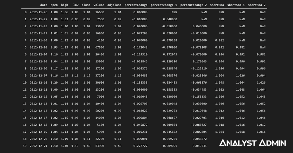
data.reset_index(inplace=True, drop=True)Now we calculate SMA using the rolling and mean operations of a Pandas series. The “5” below is for the number of days. If we want to create a Long SMA we can use something like “100” days instead of “5”. However, I will stick with a small number so that the effect can be viewed in a small window of data.
# create a simple moving average using rolling calculations
data['shortSma'] = data['close'].rolling(5).mean()
data.head(10)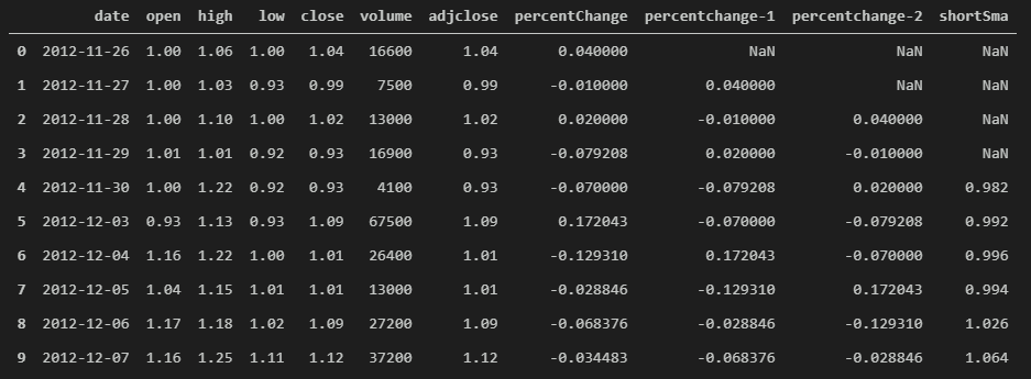
Notice the first 4 days (index 0-3) do not have a “shortSma” that’s because each of those days did not have enough days going back to calculate the rolling(5).
Now that we have SMA we can shift it to create two new features.
# shift the SMA so that a particular day knows the SMA of the previous day
data['shortSma-1'] = data['shortSma'].shift(1)
data.head(10)
# add a feature for the SMA from two days ago
data['shortSma-2'] = data['shortSma'].shift(2)
data.head(10)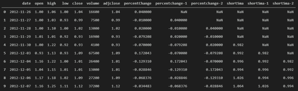
That’s it for new features. Now we can cleanup the dataframe by removing all the NaNs.
#trim the obervations with missing calculated data
data.dropna(inplace=True)
data.head(10)
The function above will remove all observations where at least one feature contains a NaN, so be careful. You can use the “subset” argument to only drop observations where only specific columns contain NaN if you are not sure about your data.
Now let’s separate the data into an X and y (features & target vector).
# separate features
features = ['percentchange-1', 'percentchange-2', 'shortSma-1', 'shortSma-2']
X = data[features]

# separate the target vector
y = data['percentChange']
We will then scale the X so that when we train our linear regression model we can analyze the coefficients in the same scale. I will use a scikit-learn function called “scale” within the preprocessing library.
# scale the features with unit-mean standard deviation
X = pd.DataFrame(preprocessing.scale(X), index = X.index, columns = X.columns)
Next, I will use the scikit-learn “train_test_split” function to divide my data into training and testing sets randomly. The testing size is set to “0.2” or 20% which means I will be training the model on 80% of the dataset which is a safe split for linear regression given the dataset.
# create training and testing sets by splitting the full dataset
X_train, X_test, y_train, y_test = train_test_split(X, y, test_size=0.2, random_state=1)
Special note, this will generate two new dataframes and two new series, X_train, X_test, y_train, y_test, respectively.
Now the data is 100% ready for a machine learning algorithm. From this point on we jump into a linear regression algorithm to train and test the model. Special note, in the real world you will probably not be using a linear regression algorithm to predict the stock market. I’m using linear regression here for the sake of simplicity.
# create a linear regression object
my_linreg = LinearRegression()
To fit the model to the training data we will use the “fit” function and pass in our training data.
# fit the linear regression object to the training data
my_linreg.fit(X_train, y_train)
Now that the model is fit, we can see the coefficients of each feature. In general, the coefficient with the highest absolute value is the most correlated with the target vector. Also, positive coefficients are positively correlated while negative coefficients are negatively correlated with the target vector.
# print out the linear regression coefficients
print(my_linreg.coef_)
Out: [-1.83861458e-03 3.81734250e-06 -1.14631594e-01 1.14308136e-01]To see which feature has the most correlation we can create a new dataframe with coefficients and column names. I’ve also gone ahead and taken the absolute value and sorted the data.
# put coefficients in dataframe, take absolute value and sort
coffDf = pd.DataFrame(list(zip(X.columns,np.absolute(my_linreg.coef_))), columns=['Feature','Coefficient'])
coffDf.sort_values('Coefficient', ascending=False)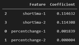
Notice how shortSma-1 has the highest absolute value! That means that shortSma-1 has the highest correlation with the percent change (target vector). This type of analysis can be used to create more relevant features and to understand what value each feature is bringing to the model.
Now let’s use the trained model to predict on the testing set.
# make predictions on the testing set
y_prediction = my_linreg.predict(X_test)
print(y_prediction)
Out:
[-1.29455651e-03 -3.96322055e-03 6.59419710e-04 -2.59123916e-03
1.95729587e-03 3.82718757e-03 -4.94597329e-03 2.88532953e-03
-2.18723623e-03 -2.78564265e-03 2.24264894e-03 -2.14085641e-03
5.18296801e-03 -5.71483878e-03 -5.88216743e-04 3.16728605e-04
-2.61084259e-04 2.01959059e-03 -2.34961277e-03 -2.43163486e-03
1.79225243e-03 2.64776225e-03 3.02945196e-03 -1.45447217e-04
3.71679868e-03 2.23369595e-03 -1.06319715e-03 2.11801614e-03
-7.81162087e-03 8.04337714e-03 4.67753488e-04 2.96275248e-04
5.88536554e-03 6.41958589e-03 -5.19879732e-05 1.28886416e-03
2.00956319e-03 -2.68709458e-03 -6.09952132e-03 -3.79141647e-03
3.58422779e-03 2.88474576e-03 1.53894669e-03 2.13184595e-04
2.46513006e-04 4.40403505e-03 -1.72738960e-03 1.23677597e-03
-2.92647785e-04 -2.72097674e-03 5.93572234e-03]Now that we have the test predictions we can calculate the mean squared error (MSE). Followed by a square root of the MSE to arrive at RMSE.
# calculate the mean squared error of the predictions
mse = metrics.mean_squared_error(y_test, y_prediction)

# take the square root of MSE to get Root Mean Squared Error (RMSE)
rmse = np.sqrt(mse)

print(rmse)
Out: 0.044721137880460754Now, as you can see our RMSE is 0.04 which means our predictions could be off by 4%. That’s not very good for trading but it can provide a baseline to compare against. To improve the results, we can try adding more features and observations, trying different machine learning algorithms, and optimizing the parameters of those algorithms. I hope this gives you an idea of how we go from bare stock trading data to refined machine learning data!
Thank you for reading!